Back to RasterLite2 Tutorials index

Tutorial: building and testing the Trieste sample

In this tutorial we'll use a more exotic raster datasource, i.e. an orthorectified scene taken from the OrbView3 satellite.
The most interesting feature of this datasource is in that the satellite's sensors captured a 16 bit Panchromatic (i.e. black & white) image; and such a configuration isn't one ordinarily supported by many non-specialized, general purpose image viewers/editors.

Step 1) downloading the OrbView3 scene

open your web browser and go to the USGS EarthExplorer web portal.
a preliminary user registration is required in order to effectively enable any download option; but it's a simple and easy step.
Please note: you can get many USGS datasets absolutely for free, under an Open Data license substantially equivalent to CC-BY (attribution).
select the ORBVIEW 3 dataset.
select coordinates near Latitude 45°39′10″N, Longitude 13°46′00″E; then start searching between the available datasets.
now select the 3V060906P0001360991A520012601472M_001604256 scene, and finally download the LEVEL 1GST package.

Step 2) retrieve all basic informations about the OrbView3 scene

$ tiffinfo 3v060906p0001360991a520012601472m_001604256_1GST.TIF
TIFF Directory at offset 0x16a1bc23 (379698211)
  Subfile Type: (0 = 0x0)
  Image Width: 8326 Image Length: 22791
  Resolution: 1, 1
  Bits/Sample: 16
  Sample Format: unsigned integer
  Compression Scheme: None
  Photometric Interpretation: min-is-black
  Orientation: row 0 top, col 0 lhs
  Samples/Pixel: 1
  Rows/Strip: 1
  Planar Configuration: single image plane
  Tag 33550: 1.010000,1.010000,0.000000
  Tag 33922: 0.000000,0.000000,0.000000,400387.050653,5075006.239869,0.000000
  Tag 34735: 1,1,0,5,1024,0,1,1,1025,0,1,1,2052,0,1,9001,2054,0,1,9102,3072,0,1,
32633
  Tag 34737: WGS-84
$

As reported by the tiffinfo tool, this TIFF file contains a 8,326 x 22,791 raster; the suggested photometric interpretation is Grayscale (min-is-black), and pixel values are of the UINT16 type (Sample Format: unsigned integer and Bits/Sample: 16).

$ listgeo 3v060906p0001360991a520012601472m_001604256_1GST.TIF
Geotiff_Information:
   Version: 1
   Key_Revision: 1.0
   Tagged_Information:
      ModelTiepointTag (2,3):
         0                 0                 0
         400387.050653227  5075006.239869    0
      ModelPixelScaleTag (1,3):
         1.01              1.01              0
      End_Of_Tags.
   Keyed_Information:
      GTModelTypeGeoKey (Short,1): ModelTypeProjected
      GTRasterTypeGeoKey (Short,1): RasterPixelIsArea
      GeogLinearUnitsGeoKey (Short,1): Linear_Meter
      GeogAngularUnitsGeoKey (Short,1): Angular_Degree
      ProjectedCSTypeGeoKey (Short,1): PCS_WGS84_UTM_zone_33N
      End_Of_Keys.
   End_Of_Geotiff.

PCS = 32633 (WGS 84 / UTM zone 33N)
Projection = 16033 (UTM zone 33N)
Projection Method: CT_TransverseMercator
   ProjNatOriginLatGeoKey: 0.000000 (  0d 0' 0.00"N)
   ProjNatOriginLongGeoKey: 15.000000 ( 15d 0' 0.00"E)
   ProjScaleAtNatOriginGeoKey: 0.999600
   ProjFalseEastingGeoKey: 500000.000000 m
   ProjFalseNorthingGeoKey: 0.000000 m
GCS: 4326/WGS 84
Datum: 6326/World Geodetic System 1984
Ellipsoid: 7030/WGS 84 (6378137.00,6356752.31)
Prime Meridian: 8901/Greenwich (0.000000/  0d 0' 0.00"E)
Projection Linear Units: 9001/metre (1.000000m)

Corner Coordinates:
Upper Left    (  400387.051, 5075006.240)  ( 13d43' 3.59"E, 45d49'17.12"N)
Lower Left    (  400387.051, 5051987.330)  ( 13d43'20.62"E, 45d36'51.43"N)
Upper Right   (  408796.311, 5075006.240)  ( 13d49'33.22"E, 45d49'21.31"N)
Lower Right   (  408796.311, 5051987.330)  ( 13d49'48.81"E, 45d36'55.59"N)
Center        (  404591.681, 5063496.785)  ( 13d46'26.58"E, 45d43' 6.42"N)
$

The listgeo tool confirms that this actually is GeoTIFF including full-referencing and that the intended Reference System is SRID=32633 (WGS 84 / UTM zone 33N); the declared pixel resolution equals to 1.01 meters on both axes (square pixels).

Step 3) creating the Trieste Coverage

$ rl2tool CREATE -db trieste.sqlite -cov trieste -smp UINT16 \
-pxl DATAGRID -cpr LZMA -srid 32633 -res 1.01

rl2_tool: request is CREATE
===========================================================
              DB path: trieste.sqlite
             Coverage: trieste
          Sample Type: UINT16
           Pixel Type: DATAGRID
      Number of Bands: 1
          Compression: LZMA (7-zip, lossless)
   Tile size (pixels): 512 x 512
                 Srid: 32633
Pixel base resolution: X=1.01 Y=1.01
===========================================================

     SQLite version: 3.8.4.2
 SpatiaLite version: 4.2.0-devel
RasterLite2 version: 0.8

Raster Coverage "trieste" successfully created

Operation CREATE successfully completed
$

Exactly as you already did in any previous tutorial you'll invoke rl2tool from the command shell.
the most relevant arguments will be explained one by one:
- -smp UINT16 this specifies the Coverage's Sample Type.
- -pxl DATAGRID this specifies the Coverage's Pixel Type.
  Please note: we'll use DATAGRID instead of GRAYSCALE because RasterLite2 doesn't supports Grayscale 16-bit.
- -cpr LZMA this specifies that all Tiles in this Coverage must be compressed using the lossless LZMA algorithm; this one is an advanced algorithm ensuring better compression than the usual DEFLATE, and effectively allows to reach compression factors as high as 1:2 or (may be) 1:3.
  It's usually quite slow during the compression, but it's noticeably fast during decompression.
  Please note: in this case using the common JPEG compression is completely out of discussion, because JPEG doesn't support 16 bit pixels.

Step 4) populating the Trieste Coverage

$ rl2tool IMPORT -db trieste.sqlite -cov trieste \
-src 3v060906p0001360991a520012601472m_001604256_1GST.TIF -pyr

rl2_tool; request is IMPORT
===========================================================
              DB path: trieste.sqlite
    Input Source path: 3v060906p0001360991a520012601472m_001604256_1GST.TIF
             Coverage: trieste
              Section: from file name
Immediately building Pyramid Levels
===========================================================

     SQLite version: 3.8.4.2
 SpatiaLite version: 4.2.0-devel
RasterLite2 version: 0.8

Importing: 3v060906p0001360991a520012601472m_001604256_1GST.TIF
------------------
    Image Size (pixels): 8326 x 22791
                   SRID: 32633
       LowerLeft Corner: X=400387.05 Y=5051987.33
      UpperRight Corner: X=408796.31 Y=5075006.24
       Pixel resolution: X=1.010000000000001 Y=1.010000000000006
  ----------
    Pyramid levels successfully built for: 3v060906p0001360991a520012601472m_001604256_1GST

Operation IMPORT successfully completed
$

You'll simply invoke rl2tool IMPORT exactly in the same way already adopted in any other previous tutorial.

Step 5) understanding Contrast Enhancement and Raster Styles

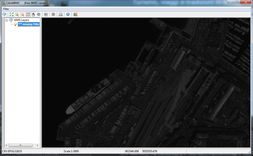
This image exemplifies how the Trieste sample will look using the plain default Style. Just a quick glance shows how this image doesn't look good at all; it's exaggeratedly dark, it looks completely unnatural and it's really difficult to be correctly interpreted. In few worlds, it definitely sucks and it's practically useless.
Just a quick recall: this is not at all an ordinary orthorectified aerial photography of the usual type; this one is a satellite digital image taken from an altitude of about 670 km and supporting 16 bit pixel values.
Most precisely, the digital sensors used by the OrbView3 satellite have an internal precision of just 11 bits, and each sample value has been opportunely padded so to adapt into a more common 16 bit integer. This image has already been carefully post-processed so to correct many original defects (removing digital noise and applying radiometric recalibration) and has been precisely orthorectified; anyway, in photographic terms it still suffers of a catastrophic under-exposure.

Conclusion: we are expected to apply some appropriate contrast enhancement method in order to finally get a decent image.
The WMS standard specifications fully support raster styling via RasterSymbolizer definitions, as disciplined by a further standard specification i.e. OGC SLD/SE 1.1.0. More specifically the following alternative Contrast Enhancement methods are made available by a standard RasterSymbolyzer:

a Gamma Value tells how much to brighten (values greater than 1.0) or dim (values less than 1.0) an image. The default GammaValue is 1.0 (no change).
Histogram means to stretch the contrast based on a histogram of how many colors are at each brightness level on input, with the goal of producing equal number of pixels in the image at each brightness level on output. This has the effect of revealing many subtle ground features.
Normalize means to stretch the contrast so that the dimmest color is stretched to black and the brightest color is stretched to white, with all colors in between stretched out linearly.
If none of Normalize, Histogram, or GammaValue are selected in a ContrastEnhancement, then no enhancement is performed.

RasterLite2 fully supports RasterSymbolizer Contrast Enhancement. The algorithms adopted by RasterLite2 exactly correspond to the ones described in these academic lecture notes; more precisely:

the non-linear Gamma Function algorithm matches a Gamma Value request.
the linear Histogram Equalization algorithm matches an Histogram request.
an hybrid Crop / Stretch approach will match a Normalize request. Crop will be applied first, so to discard all samples belonging to the first and last two percentiles; this practically means applying a cut-off < 2% and > 98% of the area under the distribution curve. And finally the Histogram Stretching algorithm will be applied.

The following practical examples will surely help to understand better.

Contrast Enhancement: Gamma Value

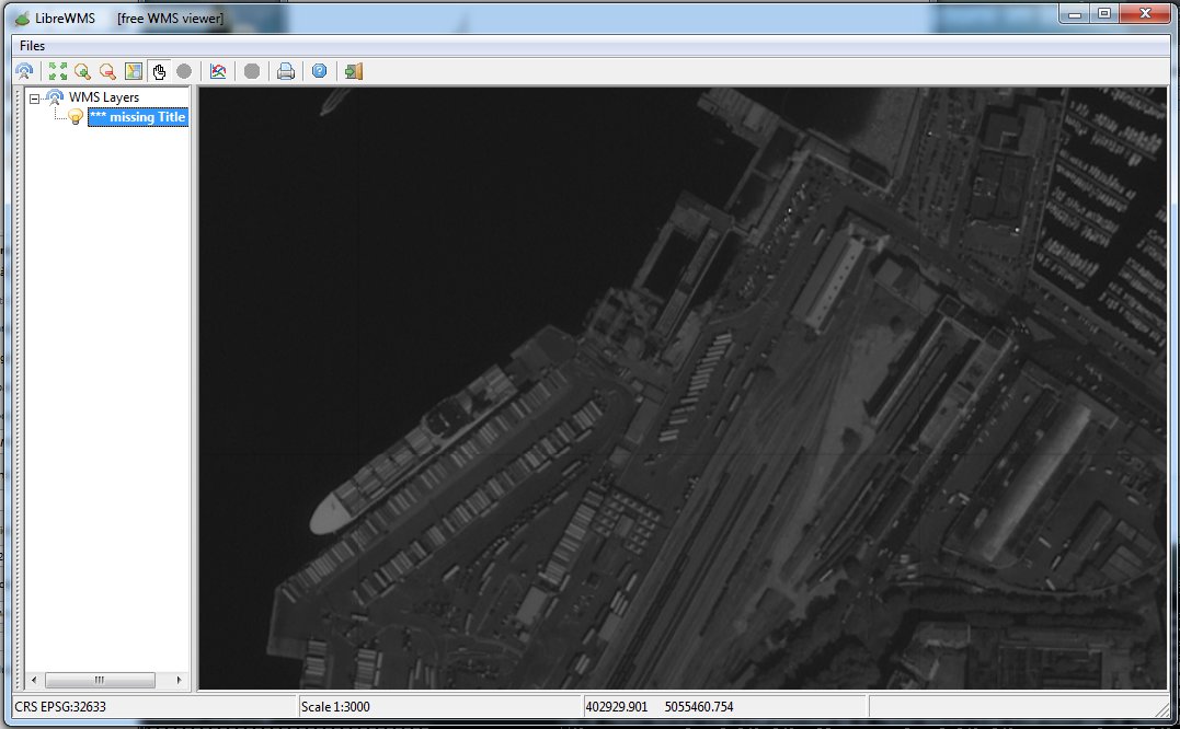
This image is an example of how the Gamma Value contrast enhancement method works. In this case we've applied a Gamma coefficient equal to 1.5 and consequently the image is now slightly brighter then before.

trieste gamma 2.0

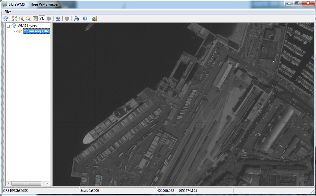
Yet another example; now the Gamma coefficient if set to 2.0 and the image is increasingly brighter.

trieste gamma 2.5

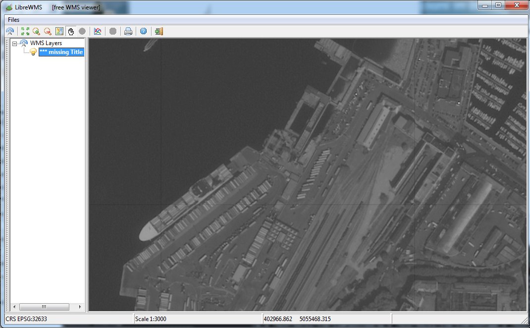
In this final example the Gamma coefficient if set to 2.5; the image is now decently bright, but starts suffering from a different issue. The contrast is now exaggeratedly flattened, and the image looks dim and washed out.
Conclusions: the GammaValue contrast enhancement method suffers from two strong disadvantages:

explicitly specifying a coefficient is strictly required; and guessing the most appropriate value could be a difficult task, and could easily vary for different images presenting different characteristics.
there is a noticeable gain in brightness, but always at the expense of a corresponding contrast flattening.
may well be that this method could be some way useful, but it's not really interesting under a more general perspective.

Contrast Enhancement: Histogram

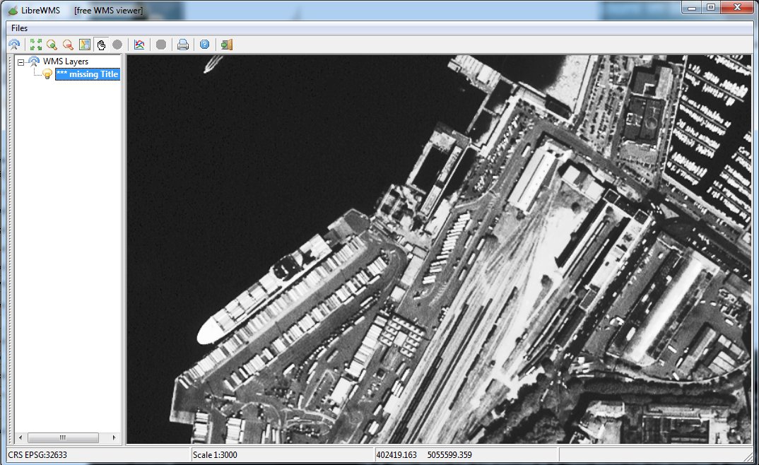
This method seems to be more interesting: it doesn't require any explicit argument and can directly support any arbitrary image. The image apparently looks reasonably natural at first glance, but if you look better paying closer attention to fine details there are still several issues. The overall contrast is now too much aggressive: many areas has become full white thus lacking any internal detail.
Conclusions: the Histogram contrast enhancement method is rather good, but it isn't perfect.

Contrast Enhancement: Normalize

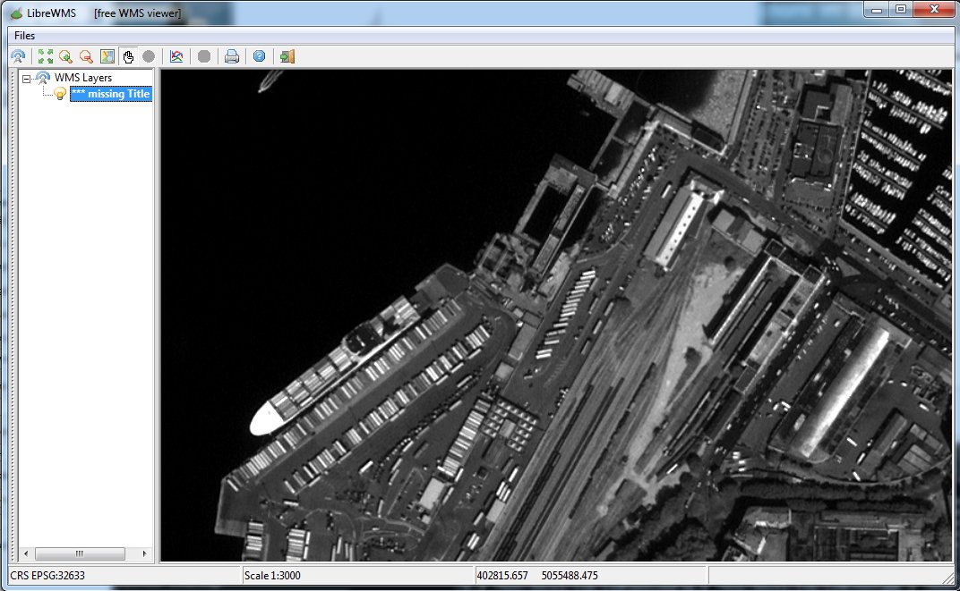
Finally we have a really natural-looking image; the overall contrast is well balanced, the image is clear and sharp, many fine-grained details are perfectly preserved and easily visible.
Conclusions: the Normalize contrast enhancement method seems to be the best available choice.

Step 6) using and understanding Band Histograms

You'll probably remember that in the previous Trento tutorial we've already examined Band Histograms.

trento band#0 histogram

This is the Histogram corresponding to the Red band of the Trento Coverage.

trento band#1 histogram

Green band.

trento band#2 histogram

Blue band.
As you can easily notice, all these histograms clearly corresponds to the classic bell curve we are expecting for any normal Gaussian distribution: and effectively the Trento sample has a fair natural-looking aspect, has a good brightness and presents a well balanced contrast.

$ rl2tool HISTOGRAM -db trieste.sqlite -cov trieste

rl2_tool; request is HISTOGRAM
===========================================================
    DB path: trieste.sqlite
   Coverage: trieste
             Histogram from Coverage-level Statistics
 Band Index: 0
Destination: ./hist_trieste_0.png
===========================================================

     SQLite version: 3.8.4.2
 SpatiaLite version: 4.2.0-devel
RasterLite2 version: 0.8

Operation HISTOGRAM successfully completed
$

Coming back to the Trieste sample; you'll now create the Coverage-level Histogram.
Please note: you can now avoid to explicitly specify the -bnd index argument, because the Trieste Coverage has just a single band.

trieste band#0 histogram

Gray band.
As you immediately notice looking at the Histogram, the Trieste sample presents an abnormal sample distribution. This Histogram is strongly compressed, i.e. quite all values are grouped in the low-end range. And this obviously explains why the first default image extracted from the Trieste Coverage was so dark and presented a catastrophic under-exposure.
We'll now examine few Histograms corresponding to the same small sized output image after applying each Contrast Enhancement method.

Contrast Enhancement: Gamma Value

Gamma value = 1.5

trieste gamma value=2.0 histogram

Gamma value = 2.0

trieste gamma value=2.5 histogram

Gamma value = 2.5

These histograms confirm our first impression: the Gamma Value method progressively shifts the mean value, but doesn't expand at all the distribution who still remains compressed; so the output image will effectively become brighter but the contrast will always remain poor.

Contrast Enhancement: Histogram

In this case too the histogram confirms our first impression: the Histogram method effectively expands the distribution, who remains anyway rather flat and consequently unnatural and not completely convincing.

Contrast Enhancement: Normalize

And finally we have an objective demonstration explaining why the Normalize method produces natural-looking images; now the histogram is still far from ideal perfection, but at least it presents a clear bell shaped distribution.

SELECT RL2_GetBandHistogramFromImage(
  RL2_GetMapImage('trieste', ST_Buffer(ST_Centroid(geometry), 640), 
  1280, 1280, 'trieste_gamma_2.5', 'image/png'), 'image/png', 0)
FROM trieste_tiles 
WHERE tile_id = 552;

Just for the sake of curiosity: all histograms representing the various Contrast Enhancement methods were captured by using SQL queries like the above one.

Step 7) creating and loading your own custom Raster Styles

7.1) downloading the Trieste styles

Just download the appropriate resource-pack from here; it contains any SLD/SE RasterSymbolizer required by this tutorial.

7.2) exploring the SLD/SE RasterSymbolizer anatomy

<?xml version="1.0" encoding="UTF-8"?>
<RasterSymbolizer version="1.1.0" 
		xsi:schemaLocation="http://www.opengis.net/se http://schemas.opengis.net/se/1.1.0/Symbolizer.xsd"
		xmlns="http://www.opengis.net/se"
		xmlns:ogc="http://www.opengis.net/ogc"
		xmlns:xlink="http://www.w3.org/1999/xlink"
		xmlns:xsi="http://www.w3.org/2001/XMLSchema-instance">
	<Name>trieste_gamma_1.5</Name>
	<Description>
		<Title>Contrast Enhancement: GammaValue=1.5</Title>
		<Abstract>a styled 16-bit grayscale raster supporting contrast enhancement; GammaValue method (coeff=1.5)</Abstract>
	</Description>
	<Opacity>1.0</Opacity>
	<ContrastEnhancement>
		<GammaValue>1.5</GammaValue>
	</ContrastEnhancement>
</RasterSymbolizer>

Any RasterSymbolizer simply is an XML Document, i.e. a text file; you can safely use any ordinary text editor in order to view and eventually modify a RasterSymbolizer:

each RasterSymbolizer is identified by its Name; both RasterLite2 and WMS require that each RasterSymbolizer supporting the same Coverage/Layer should declare a unique, non-ambiguous Name.
adding a clear Title and an optional Abstract surely is a good practice, because this way end users will easily understand the intended scope for each alternative Style eventually supporting the same Coverage/Layer. Usually the Title is expected to just contain a short summary, whilst the Abstract should be more verbose, information rich and easy to be understood.
the allowed declarations supporting ContrastEnhancement are the following ones:

	<ContrastEnhancement>
		<GammaValue>1.5</GammaValue>
	</ContrastEnhancement>

	<ContrastEnhancement>
		<Histogram />
	</ContrastEnhancement>

	<ContrastEnhancement>
		<Normalize />
	</ContrastEnhancement>

7.3a) importing all RasterSymbolizers into the DB-file

$ export "SPATIALITE_SECURITY=relaxed"
$ sqlite3 trieste.sqlite
SQLite version 3.8.4.2 2014-03-26 18:51:19
Enter ".help" for usage hints.
sqlite> .null NULL
sqlite> SELECT load_extension('mod_spatialite');
NULL
sqlite> SELECT CreateStylingTables();
1
sqlite> SELECT RegisterRasterStyledLayer('trieste',
   ...> XB_Create(XB_LoadXML('./trieste_styles/trieste_gamma_1.5.xml'), 1, 1));
1
sqlite> SELECT RegisterRasterStyledLayer('trieste',
   ...> XB_Create(XB_LoadXML('./trieste_styles/trieste_gamma_2.0.xml'), 1, 1));
1
sqlite> SELECT RegisterRasterStyledLayer('trieste',
   ...> XB_Create(XB_LoadXML('./trieste_styles/trieste_gamma_2.5.xml'), 1, 1));
1
sqlite> SELECT RegisterRasterStyledLayer('trieste',
   ...> XB_Create(XB_LoadXML('./trieste_styles/trieste_histogram.xml'), 1, 1));
1
sqlite> SELECT RegisterRasterStyledLayer('trieste',
   ...> XB_Create(XB_LoadXML('./trieste_styles/trieste_normalize.xml'), 1, 1));
1
sqlite> SELECT * FROM SE_raster_styled_layers_view;
...
sqlite> .quit
$

Please note well: explicitly setting the environment variable SPATIALIATE_SECURITY=relaxed is strictly required in any case, because you are going to invoke security sensible SQL functions directly loading external files into the DB-file.
the CreateStylingTables() SQL function will create all DB tables required in order to support SLD/SE standard styling; if these tables are eventually already been created this action will have no further consequence.
the RegisterStyledLayer() SQL function will then associate any RasterSymbolizer to the trieste Raster Coverage.
and in turn the XB_LoadXML() SQL function will then load and the XML external documents from the local file-system.
Please note: only RasterSymbolizers presenting a very strict conformance to SLD/SE 1.1.0 standard specifications will be accepted, because a formal XSD Schema validation will be preliminary tested.

coverage_name	style_id	name	title	abstract	style	schema_validated	schema_uri
trieste	0	trieste_gamma_1.5	Contrast Enhancement: GammaValue=1.5	a styled 16-bit grayscale raster supporting contrast enhancement; GammaValue method (coeff=1.5)	XmlBLOB-RasterStyle sz=599 (XMLsz=700) SchemaValidated	1	http://schemas.opengis.net/se/1.1.0/Symbolizer.xsd
trieste	1	trieste_gamma_2.0	Contrast Enhancement: GammaValue=2.0	a styled 16-bit grayscale raster supporting contrast enhancement; GammaValue method (coeff=2.0)	XmlBLOB-RasterStyle sz=597 (XMLsz=700) SchemaValidated	1	http://schemas.opengis.net/se/1.1.0/Symbolizer.xsd
trieste	2	trieste_gamma_2.5	Contrast Enhancement: GammaValue=2.5	a styled 16-bit grayscale raster supporting contrast enhancement; GammaValue method (coeff=2.5)	XmlBLOB-RasterStyle sz=599 (XMLsz=700) SchemaValidated	1	http://schemas.opengis.net/se/1.1.0/Symbolizer.xsd
trieste	3	trieste_histogram	Contrast Enhancement: Histogram	a styled 16-bit grayscale raster supporting contrast enhancement; Histogram method	XmlBLOB-RasterStyle sz=558 (XMLsz=666) SchemaValidated	1	http://schemas.opengis.net/se/1.1.0/Symbolizer.xsd
trieste	4	trieste_normalize	Contrast Enhancement: Normalize	a styled 16-bit grayscale raster supporting contrast enhancement; Normalize method	XmlBLOB-RasterStyle sz=557 (XMLsz=666) SchemaValidated	1	http://schemas.opengis.net/se/1.1.0/Symbolizer.xsd

This table represents the actual content of the DB View named SE_raster_styled_layers_view after registering all RasterSymbolizers, exactly as the reported by the SELECT * FROM SE_raster_styled_layers_view SQL query.
Now you are finally ready to perform a practical test based on the trieste sample.

7.3b) importing all RasterSymbolizers (alternative easier way)

If you dislike invoking so many complex SQL statements, you'll probably be happy to learn that the same identical task could be eventually performed in a more user friendly way by using spatialite_gui. Please consult the appropriate documentation

Step 8) testing the Trieste sample (and playing with Styles)

As you've already done in any previous tutorial you can now directly test the Trieste Coverage by publishing a standard WMS service.
You simply have to start the wmslite light-weight server, then connecting some WMS viewer (e.g. LibreWMS) to the service being published on localhost aka IP address 127.0.0.1, port 8080.

trieste WMS #1

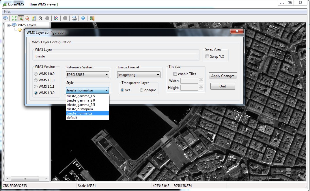
You can freely switch from a Style to another one.

trieste WMS #2

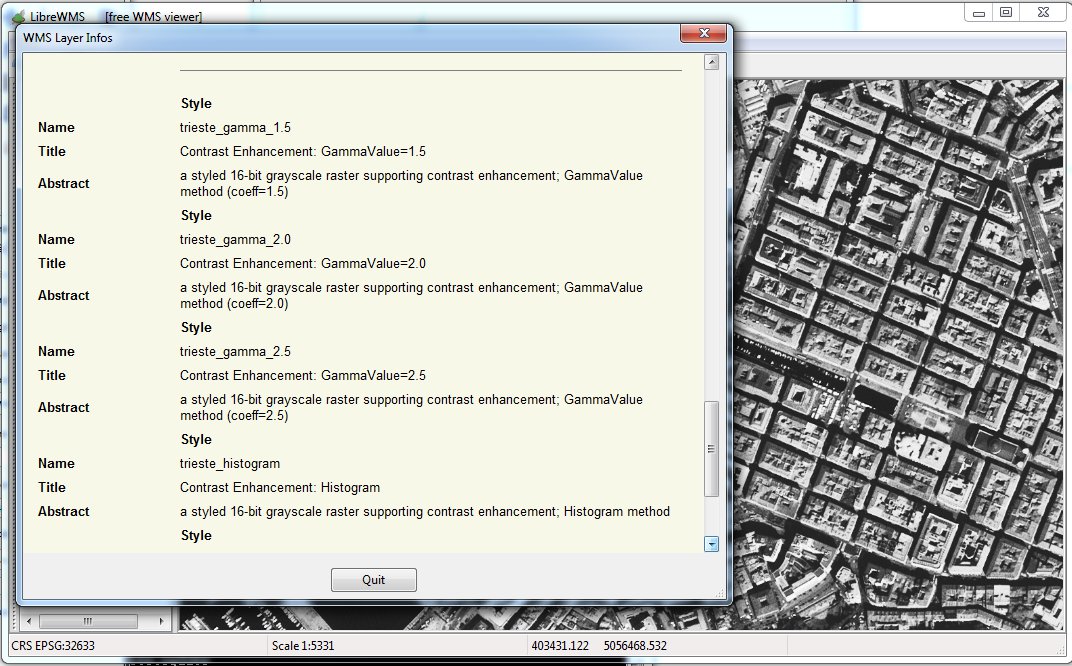
And you can read full informations supporting each single Style by consulting the WMS Metadata.

Back to RasterLite2 Tutorials index