Many hyperlinks are disabled.
Use anonymous login
to enable hyperlinks.
Overview
| Artifact ID: | 9eadd9d129d067f2d997abee4dad37cf84c9810c |
|---|---|
| Page Name: | VirtualRouting |
| Date: | 2018-04-07 15:15:00 |
| Original User: | sandro |
| Parent: | 49de9a510c9200f130f294494a508987eeadfa0c (diff) |
| Next | e4ff52035a120a693d7574d657a4620dfca584c1 |
Content
Table of Contents
1 - Introduction2 - The sample/test DB
3 - Creating VirtualRouting Tables
4 - Solving classic Shortest Path problems
5 - Solving multi-destination Shortest Path problems
6 - Solving TSP (traveling salesman) problems
1 - Introduction
Previous versions of SpatiaLite traditionally supported a pure SQL routing module that was named VirtualNetwork.Since version 5.0.0 a brand new routing module (more advanced and sophisticated) is available, that is called VirtualRouting.
The now obsolete VirtualNetwork is still supported by version 5.0.0 so as to not cause an abrupt break to already existing applications, but will presumably be discontinued in future versions.
Using VirtualRouting instead of VirtualNetwirk is warmly recommended for any new development.
Theoretical foundations - an ultra-quick recall
All Routing algorithms (aka Shortest Path algorithms) are based on the mathematics of the Graph theory or to be more precise: on Weighted Graphs.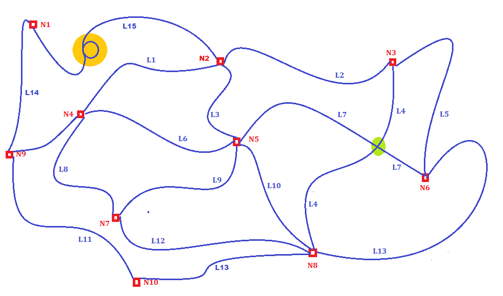
A topologically valid Network is a dataset that fulfills the following requirements:
- All items in the dataset are called Links (aka Arcs), and are expected to represent some oriented connection joining two Nodes.
Example: in the above figure Link L3 connects Nodes N2 and N5. - So all Links are always expected to explicitly reference a Start-Node (aka Node-From) and an End-Node (aka Node-To).
- Links are always oriented, and their natural direction is From-To:
- in an unidirectional Network each Link is an one-way connection.
If the connection is available in the opposite direction a second Link must be explicitly declared.
Example: Link X1 goes from Node A to Node B, and Link X2 goes from Node B to Node A. - in a bidirectional Network all Links are assumed to establish a connection in both directions.
Definiting an one-way connection requires an appropriate attribute to be set (see below).
- in an unidirectional Network each Link is an one-way connection.
- The Start- and End-Node could eventually be the same, and in this case we'll have a self-closed Link.
- Network's Links can eventually define a linear Geometry (LINESTRING) going from the Start-Node to the End-Node, but this is an optional feature, not a mandatory requirement.
- What is absolutely mandatory is that each Link must explicitly reference its Nodes.
- Links are always oriented, and their natural direction is From-To:
- A Network supporting Geometries is a Spatial Network; otherwise a Network lacking any Geometry is a Logical Network.
- In a Spatial Network all Links must have a corresponding Geometry.
- In a Logical Network all Links are strictly forbidden to have any Geometry.
- In a Spatial Network both the StartPoint and EndPoint of each Link's LINESTRING are always expected to exactly coincide with the corresponding Nodes.
- In a Spatial Network all references to the same Node by different Links must be an exact match.
Example: Node N5 is shared by Links L3, L6, L7, L9 and L10, so all their corresponding LINESTRINGS are expected to have the corresponding extremity (Start- or End-, depending on the orientation) points that must exactly match the other.
A topological inconsistency exists if any of these conditions are not satisfied, which leads to an invalid Network. - In a Spatial Network two
- Accordingly to the above premises, Nodes are never expected to be explicitly declared in a separate Table.
Just a single Table declaring all Links is required in order to fully define a topologically valid Network.
All the Nodes can then be easily extracted from the Links' definitions and the coordinates for each Node can be directly set by extracting the extreme Point of the corresponding Linestrings.
If any mismatch is detected this surely means that the Network is invalid. - A Link may legitimately self-intersect itself (e.g. forming a loop), as shown in the above figure by Link L15 (orange spot).
- Two Links may legitimately intersect where no Node exists, as exemplified on the above figure by Links L4 and L7 (green spot).
This usually happens when one of the two Links overpasses the other, or where some technical restriction exists (e.g. two insulated wires in an Electrical Network). - Links aren't strictly required to be associated with any specific attribute, but the following attributes are almost universally supported:
- a name identifying the Link.
Examples: the road toponym in a road network, or the river name in an hydrographic network. - one (or even more) appropriate cost value(s).
Example: the time required to traverse the Link (may be distinguished between pedestrians, bicycles, cars, lorries and so on). - a pair of boolean flags (from-to and to-from) are intendend to specify if the Link can be traversed on both directions or just in one (one-way).
- a name identifying the Link.
Logical conclusions
Any topologically valid Network (irrespective of whether it is a Spatial or Logical type) is a valid Graph.A Network allowing the support (direct or indirect) of some appropriate cost value is a valid Weighted Graph, and can consequently support Routing algorithms.
All Routing algorithms are intended to identify the Shortest Path solution connecting two Nodes in a weighted graph (aka Network).
Note: the term Shortest Path can be easily misunderstood.
Due to historical reasons the most common application field for Routing algorithms is related to Road Networks, but also many other kinds of Networks exist:
- Hydrographic Networks.
- Gas / Water / Oil Networks.
- Electrical Networks.
- Telecomunication Networks.
- Social or Economical Networks representing relationships between individuals or companies.
- Epidemiological Networks representing the propagation of infective diseases between individuals or groups.
In all the above cases we certainly have valid Networks supporting Routing algorithns, but not all of them can imply something like a spatial distance (geometric length) or a travel time.
In the most general acception costs can be represented by any reasonable physical quantity.
So a more generalized definition is assuming that Routing algorithms are intended to identify lesser cost solutions on a weighted graph.
The exact interpretation of the involved costs (aka weights) strictly depends on the very specific nature of each Network.
The Dijkstra's algorithm
This well known algorithm isn't necessarily the fastest one, but it always ensures full correctness:- Any Node-to-Node connection identified by Dijkstra's is certainly ensured to be optimal.
In other words, no connetction presenting a lower cost can conceptually exist. - When Dijsjtra's fails to identify a solution this surely means that no solution is possible.
The A* algorithm
Many alternative Routing algorithms have been invented during the years.All them are based on heuristic assumptions and are intended to be faster than Dijkstra's, but none of them can ensure full correctness as Dijkstra's does.
The A* algorithm applies a mild heuristic optimization, and can be a realistic alternative to Dijkstra's in many cases.
2 - The sample/test DB
You are expected to follow the current tutorial about VirtualRouting by directly testing all SQL queries discussed below on behalf of the sample/test DB that you can download from hereThe sample DB contains the full road network of Tuscany Region (Italy) (Iter.Net dataset) kindly released under the CC-BY-SA 4.0 licence terms.
The contents stored into the sample database were opportunely rearranged, and are still subject to the initial CC-BY-SA 4.0 clauses (derived work).
- all road names are stored within the toponyms Table.
the same road name could be used in different Municipalities, so the toponyms Table relationally references the municipalities Table (via PRIMARY / FOREIGN KEY relationships). - the roads Spatial Table contains about 380,000 Links, and has the following columns:
- id: unique identifier of each Link (PRIMARY KEY).
- node_from and node_to: Node identifiers. The original Iter.Net dataset adopts very long an complex alphanumeric Node codes; the integer Node IDs were obtained by calling the CreateRoutingNodes() SQL function discussed in a following section.
- id_toponym: relational reference to the corresponding road name contained into the toponyms Table (FOREIGN KEY).
- speed_kmh: the estimated average speed supported by the Link, expressed in km/h.
Note: negative speeds intend a forbidden Link. - oneway_fromto and oneway_tofrom: boolean flags intended to state if a Link can be traversed in both directions or just in a single direction (one-way).
Note: all Links declaring oneway_fromto=0 and oneway_tofrom=0 are intended to be always forbidden. - cost: the time expressed in seconds required to traverse each Link.
Note #1 all costs were calculated accordingly to the following formula: cost = ((ST_Length(geom) / 1000.0) / speed_kmh) * 3600.0
Note #2 all 86,400.0 cost values (equivalent to 1 day) approximate an infinitive cost thus intending a forbidden Link. - geom: a 3D Linestring representing the Geometry of each Link.
Note: the original Iter.Net dataset is just 2D; elevations (Z coordinates) were interpolated by draping the dataset over an orographic DEM (10m X 10m cells)
- the roads_vw Spatial View is just intended to fully resolve all relational references between roads, toponyms and municipalities, thus allowing for easier SQL queries.
- the house_nr Spatial Table contains about 1,480,000 House Numbers, and has the following columns:
- id: unique identifier of each House Number (PRIMARY KEY).
- id_road: relational reference to the corresponding Link contained into the roads Table (FOREIGN KEY).
- label: the textual label fully qualifying each House Number.
- geom: a 3D Point representing the Geometry of each House Number.
Note #1: also in this case all elevations (Z coordinates) were interpolated by draping the dataset over the same DEM as above.
Note #2: strictly specking the House Numbers are not part of the Road Network; they are include into the sample/test database just because they'll be useful in some of the examples explained in below paragraphs.
- the house_nr_vw Spatial View is just intended to fully resolve all relational references between house_nr, roads, toponyms and municipalities, thus allowing for easier SQL queries.
3 - Creating VirtualRouting Tables
All VirtualRouting queries are based on some VirtualRouting Table, and in turn any VirtualRouting Table is based on some appropriate Binary Data Table supporting an efficient representation of the underlying Network.So we'll start first by creating such tables.
The old and now superseded VirtualNetwork required using a separate CLI tool (spatialite_network) in order to properly initialize a VirtualNetwork Table and its companion Binary Data Table; alternatively spatialite_gui supported a GUI wizard for the same task. Since version 5.0.0 now SpatiaLite directly supports a specific CreateRouting() SQL function.
SELECT CreateRouting('byfoot_data', 'byfoot', 'roads_vw', 'node_from', 'nodeto', 'geom', NULL);

SELECT CreateRouting_GetLastError();
------------------------------------
ToNode Column "nodeto" is not defined in the Input Table
Note: this first query (based on the reduced form of CreateRouting) contains an intended error causing a failure and thus raising an exception.CreateRouting() can fail for multiple reasons, and by calling CreateRouting_GetLastError() you can easily identify the exact reason why the most recent call to CreateRouting() failed.
SELECT CreateRouting('byfoot_data', 'byfoot', 'roads_vw', 'node_from', 'node_to', 'geom', NULL, 'toponym', 1, 1);
-------------
1

SELECT CreateRouting_GetLastError();
------------------------------------
NULL
This second attempt is finally successful, and now CreateRouting() returns 1 (aka TRUE), and as you can easily check now the Database contains two new Tables: byfoot and byfoot_data.Note: after a successful call to CreateRouting() CreateRouting_GetLastError() will always return NULL.
You've just used one of the partially reduced form of CreateRouting(); let's see in more depth all the arguments and their meaning:
- byfoot_data: the name of the Network Binary Data Table to be created.
- byfoot: the name of the VirtualRouting Table to be created.
- roads_vw: the name of the Spatial Table or Spatial View representing the underlying Network.
Note: in this case we actually used a Spatial View. - node_from: name of the column (in the above Table or View) expected to contain node-from values.
- node_to: name of the column (in the above Table or View) expected to contain node-to values.
- geom: name of the column (in the above Table or View) expected to contain Linestrings.
We could have legitimately passed a NULL value for this argument in the case of a Logical Network. - NULL: name of the column (in the above Table or View) expected to contain cost values.
In this case we have passed a NULL value, and consequently the cost of each Link will be assumed to be represented by the geometric length of the corresponding Linestring.
Note #1: in the case of Networks based on longitudes and latitudes (aka geographic Reference Systems) the geometry length of all Linestrings will be precisely measured on the ellipsoid by applying the most accurate geodesic formulae and will be consequently expressed in meters. In any other case (projected Reference Systems) lengths will be expressed in the measure unit defined by the Reference System (e.g. meters for UTM projections and feet for NAD-ft projections).
Note #2: the geom-column and cost-column arguments are never allowed to be NULL at the same time. - toponym: name of the column (in the above Table or View) expected to contain road-name values.
It could be legitimately set to NULL if all Links are anonymous. - 1: a boolean flag intended to specify if the Network must support the A* algorithm or not (set to TRUE by default).
- 1: a boolean flag intended to specify if all Network's Links are assumed to be bidirectional or not (assumed to be TRUE by default).
Technical noteThe internal encoding adopted by the Binary Data Table is unchanged and is the same for both VirtualNetwok and VirtualRouting.You can safely base a VirtualRouting Table on any existing Binary Data Table created by the spatialite-network CLI tool, exactly as you can base a VirtualNetwork Table on any Binary Data Table created by the CreateRouting() SQL function.
CREATE VIRTUAL TABLE test_network USING VirtualNetwork('some_data_table');

CREATE VIRTUAL TABLE test_routing USING VirtualRouting('some_data_table');
In order to manually create your Virtual Tables you just have to execute an appropriate CREATE VIRTUAL TABLE ... USING Virtual... (...) statement.
WarningIn the case of Spatial Networks based on any geographic Reference System (using longitudes and latitudes) there is an important difference between Binary Data Tables created by the spatialite_network GUI tool and Binary Data Tables created by the CreateRouting() SQL function when costs are implicitly based on the geometric length of the Link's Linestring:
|
SELECT CreateRouting('bycar_data', 'bycar', 'roads_vw', 'node_from', 'node_to', 'geom', 'cost', 'toponym', 1, 1, 'oneway_fromto', 'oneway_tofrom', 0);
--------------------
1
After calling yet another time CreateRouting() now the Database contains two further Tables: bycar and bycar_data.This time you've used the complete form of CreateRouting(); let's see in more depth all the arguments and their meaning:
- bycar_data: same as above.
- bycar: same as above.
- roads_vw: same as above.
- node_from: same as above.
- node_to: same as above.
- geom: same as above.
- cost: same as above. In this case we have referenced a column preloaded with values corresponding to the time measured in seconds required to traverse each Link.
- toponym: same as above.
- 1: same as above (A* enabled).
- 1: same as above (bidirectional Links).
- oneway_fromto: name of the column (in the above Table or View) expected to contain boolean flags specifying if each Link can be traversed in the from-to direction or not.
- oneway_tofrom: name of the column (in the above Table or View) expected to contain boolean flags specifying if each Link can be traversed in the to-from direction or not.
Note #1: both from-to and to-from column names can be legitimately set as NULL if no one-way restrictions apply to the current Network.
Note #2: Networks of the unidirectional type are never enabled to reference one-way columns (they should always be set to NULL). - 0: a boolean flag intending an overwrite authorization.
- If set to FALSE an exception will be raised if the Binary Data Table and/or the VirtualRouting Table do already exist.
- If set to TRUE eventually existing Tables will be preventively dropped immediately before starting the execution of CreateRouting().
Highlight: where you areYou've just created two VirtualRouting Tables based on different settings; both them are perfectly valid and reasonable, but they are intended for different purposes:
Conclusion: a single VirtualRouting Table can't be able to adequately support support the specific requirements and expectations of different users. Defining more Routing Tables with different settings for the same Network usually is a good design choice leading to more realistic results. |
Utility function for automatically setting NodeFrom and NodeTo IDs
Sometimes it could eventually happen to encounter some Spatial Network representation being fully topologically consistent but completely lacking any definition about NodeFrom and NodeTo identifiers.In this specific case you can successfully recover a perfectly valid Network by calling the CreateRoutingNodes() SQL function.
SELECT CreateRoutingNodes(NULL, 'table_name', 'geom', 'node_from', 'node_to');
_________________________
1
Let's examine all arguments and their meaning:
- NULL: name of the Attached-DB containing the Spatial Table.
It can be legitimately set to NULL, and in this case the MAIN DB is assumed. - table_name: name of the Spatial Table.
- geom : name of the column ((in the above Table) containing Linestrings.
- node_from: name of the column to be added to the above Table and populated with appropriate NodeFrom IDs.
- node_to: name of the column to be added to the above Table and populated with appropriate NodeTo IDs.
Note: both NodeFrom and NodeTo columns should not be already defined in the above Table.
Note: you can call CreateRouting_GetLastError() so to precisely identify the cause accounting for failure.
Handling dynamic NetworksSometimes it happens that a Network could be subject to rather frequent changes: some new Links require to be added, obsolete Links require to be removed, other Links may assume a different Cost, one-ways could be reversed, the discipline of pedestrian areas could be modified and so on.A VirtualRouting Table is always based on a companion Binary Data Table, that is intrinsically static, and consequently you are required to re-create both them from time to time in order to support all recent changes affecting the underlaying Network. The optimal frequency for cyclically refreshing the Routing Tables strictly depends on specific requirements, but the two overall approaches are commonly adopted:
|
Warning: how to correctly drop Network TablesWhen dropping a VirtualRouting Table and its companion Binary Data Table following the correct sequence of SQL commands is paramount.Failing to strictly respect the expected sequence will surely cause you several troubles and severe headaches, and will possibly lead to an irremediably corrupted database.
|
4 - Solving classic Shortest Path problems
The most classic Shortest Path problem requires to identify the optimal connection between an Origin Node and a Destination Node.We can easily translate such a problem into a simple SQL query targeting some VirtualRouting Table.
SELECT *
FROM byfoot
WHERE NodeFrom = 178731 AND NodeTo = 183286;
| Algorithm | Request | Options | Delimiter | RouteId | RouteRow | Role | LinkRowid | NodeFrom | NodeTo | PointFrom | PointTo | Tolerance | Cost | Geometry | Name |
|---|---|---|---|---|---|---|---|---|---|---|---|---|---|---|---|
| Dijkstra | Shortest Path | Full | , [dec=44, hex=2c] | 0 | 0 | Route | NULL | 178731 | 183286 | NULL | NULL | NULL | 300.912208 | BLOB sz=272 GEOMETRY | NULL |
| NULL | NULL | NULL | NULL | 0 | 1 | Link | 224014 | 178731 | 182885 | NULL | NULL | NULL | 94.812424 | NULL | VIA PIETRO ARETINO |
| NULL | NULL | NULL | NULL | 0 | 2 | Link | 224446 | 182885 | 178880 | NULL | NULL | NULL | 69.727726 | NULL | VIA MARGARITONE |
| NULL | NULL | NULL | NULL | 0 | 3 | Link | 224414 | 178880 | 183286 | NULL | NULL | NULL | 136.372057 | NULL | VIA MARGARITONE |
Let's quickly examine the resultset returned by the above Routing query:
- the first row (aka header row) has a special interpretation, and is intended to summarize the travel solution as a whole.
- all the following rows represent a single Link required to build the solution (optima path); Links are ordered accordingly to the travel direction connecting the Origin and the Destination.
- columns Algorithm, Request, Options, Delimiter, PointFrom, PointTo, Tolerance and Geometry are always set to NULL except that in the first row of the resultset:
- column Algorithm accounts for the Routing Algorithm used by the current query (Dijkstra's or A*).
- column Request specifies the exact nature of the current query (in this specific case Shortest Path).
- we'll ignore for now columns Options, Delimiter, PointFrom, PointTo and Tolerance: their respective meanings will be explained in following paragraphs.
- column Geometry contains a LINESTRING representation of the whole travel solution.
Note: on Logical Networks (not supporting Geometries) Geometry will always be NULL.
- we'll ignore for now column RouteId; its meaning will be explained in following paragraphs.
- column RouteRow simply is the progressive number of the row in the travel solution (always 0 in the header row).
- column Role can be Route (header row) or Link (all following rows).
- column LinkRowid references the ROWID of the corresponding Link (always set to NULL in the header row).
- column NodeFrom and NodeTo have the following interpretation:
- in the header row they correspond to he Origin and Destination Nodes.
- in all the following rows they are intended to specify the direction of the current Link.
- column Cost has the following interpretation:
- in the header tow it corresponds to the total cost of the travel.
- in all the following rows it represents the specific cost of the current Link.
- column Name contains the description of the current Link (usually a road name), and is always NULL in the header row.
Note it could be always be NULL if the VirtualRouting Table does not supports names.
Testing the return connection just requires swapping the Origin and the Destination; in this example you'll just request the meaningful columns:
SELECT RouteRow, Role, LinkRowid, NodeFrom, NodeTo, Cost, Geometry, Name
FROM byfoot
WHERE NodeTo = 178731 AND NodeFrom = 183286;
| RouteRow | Role | LinkRowid | NodeFrom | NodeTo | Cost | Geometry | Name |
|---|---|---|---|---|---|---|---|
| 0 | Route | NULL | 183286 | 178731 | 300.912208 | BLOB sz=272 GEOMETRY | NULL |
| 1 | Link | 224414 | 183286 | 178880 | 136.372057 | NULL | VIA MARGARITONE |
| 2 | Link | 224446 | 178880 | 182885 | 69.727726 | NULL | VIA MARGARITONE |
| 3 | Link | 224014 | 182885 | 178731 | 94.812424 | NULL | VIA PIETRO ARETINO |
If you remember, the byfoot VirtualRouting Table has no one-ways, and consequently the return path exactly corresponds to the first one, except in that all directions are now reversed.
Now you'll go to test the same connections, but this time you'll target the bycar VirtualRouting Table that fully supports one-ways:
SELECT RouteRow, Role, LinkRowid, NodeFrom, NodeTo, Cost, Geometry, Name
FROM bycar
WHERE NodeFrom = 178731 AND NodeTo = 183286;
| RouteRow | Role | LinkRowid | NodeFrom | NodeTo | Cost | Geometry | Name |
|---|---|---|---|---|---|---|---|
| 0 | Route | NULL | 178731 | 183286 | 101.815552 | BLOB sz=2032 GEOMETRY | NULL |
| 1 | Link | 224014 | 178731 | 182885 | 13.127874 | NULL | VIA PIETRO ARETINO |
| 2 | Link | 224446 | 182885 | 178880 | 9.654608 | NULL | VIA MARGARITONE |
| 3 | Link | 219171 | 178880 | 178732 | 7.809952 | NULL | VIA FRANCESCO CRISPI |
| 4 | Link | 219058 | 178732 | 178754 | 12.445626 | NULL | VIA FRANCESCO CRISPI |
| 5 | Link | 225888 | 178754 | 183461 | 1.599865 | NULL | VIA FRANCESCO CRISPI |
| 6 | Link | 225887 | 183461 | 182800 | 3.300590 | NULL | VIA FRANCESCO CRISPI |
| 7 | Link | 223935 | 182800 | 182799 | 6.688786 | NULL | VIALE LUCA SIGNORELLI |
| 8 | Link | 226038 | 182799 | 183456 | 1.294017 | NULL | VIALE LUCA SIGNORELLI |
| 9 | Link | 225832 | 183456 | 183444 | 2.385486 | NULL | VIALE LUCA SIGNORELLI |
| 10 | Link | 225831 | 183444 | 183554 | 3.160662 | NULL | VIALE LUCA SIGNORELLI |
| 11 | Link | 225765 | 183554 | 183954 | 7.469917 | NULL | VIALE LUCA SIGNORELLI |
| 12 | Link | 225766 | 183954 | 183905 | 3.236389 | NULL | VIALE LUCA SIGNORELLI |
| 13 | Link | 225979 | 183905 | 183626 | 13.983629 | NULL | STRADA SENZA NOME |
| 14 | Link | 224905 | 183626 | 183128 | 5.627358 | NULL | STRADA SENZA NOME |
| 15 | Link | 224897 | 183128 | 183286 | 10.030792 | NULL | VIA MARGARITONE |
SELECT RouteRow, Role, LinkRowid, NodeFrom, NodeTo, Cost, Geometry, Name
FROM bycar
WHERE NodeTo = 178731 AND NodeFrom = 183286;
| RouteRow | Role | LinkRowid | NodeFrom | NodeTo | Cost | Geometry | Name |
|---|---|---|---|---|---|---|---|
| 0 | Route | NULL | 183286 | 178731 | 103.305259 | BLOB sz=944 GEOMETRY | NULL |
| 1 | Link | 224414 | 183286 | 178880 | 18.882285 | NULL | VIA MARGARITONE |
| 2 | Link | 219171 | 178880 | 178732 | 7.809952 | NULL | VIA FRANCESCO CRISPI |
| 3 | Link | 219058 | 178732 | 178754 | 12.445626 | NULL | VIA FRANCESCO CRISPI |
| 4 | Link | 224538 | 178754 | 181972 | 7.047784 | NULL | VIA ANTONIO GUADAGNOLI |
| 5 | Link | 222575 | 181972 | 181971 | 1.852283 | NULL | VIA ANTONIO GUADAGNOLI |
| 6 | Link | 224967 | 181971 | 182891 | 14.273185 | NULL | VIA ANTONIO GUADAGNOLI |
| 7 | Link | 224168 | 182891 | 183057 | 6.643309 | NULL | VIA MACALLE' |
| 8 | Link | 224167 | 183057 | 183056 | 3.151272 | NULL | VIA MACALLE' |
| 9 | Link | 224174 | 183056 | 182941 | 7.966870 | NULL | VIA RODI |
| 10 | Link | 224059 | 182941 | 182001 | 6.393747 | NULL | VIA RODI |
| 11 | Link | 222637 | 182001 | 182000 | 2.475538 | NULL | VIA PIETRO ARETINO |
| 12 | Link | 222636 | 182000 | 178731 | 14.363408 | NULL | VIA PIETRO ARETINO |
As you can easily notice, the optimal paths returned by the bycar VirtualRouting Table the paths in opposite directions strongly differ between them, and both are completely different from the path returned by querying byfoot.
A quick glance at the below map will surely help to understand better what's really happening.
This is a central area of the town of Arezzo around the archaeological ruins of the Roman Amphitheater; circulating by car is discouraged and is subject to many one-way restrictions. Not surprisingly, moving by foot is the faster option.
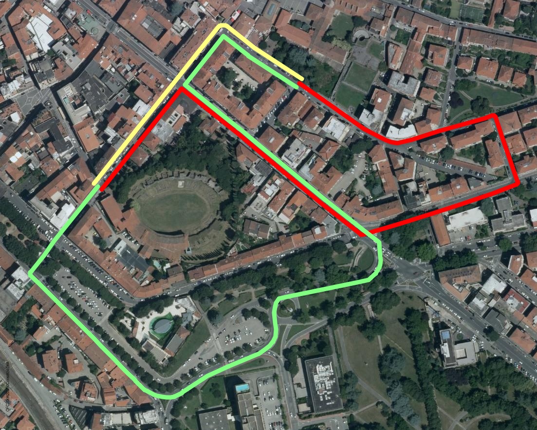
- yellow path: pedestrians
- green path: car, direct direction
- red path: car, return direction
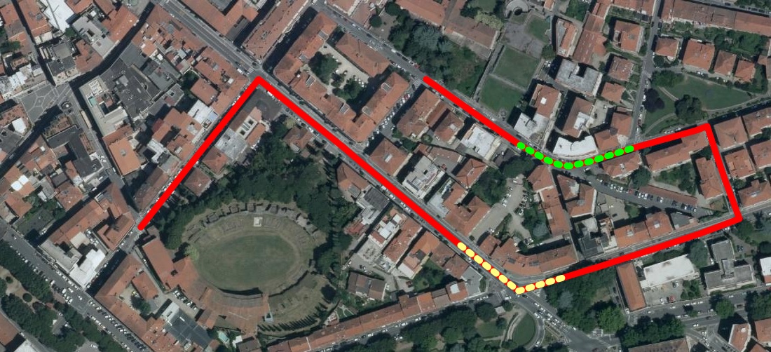
Linestrings returned by VirtualRoutingAll LINESTRING Geometries created by any VirtualRouting will always contain M values:
In other words, all Linestrings returned by VirtualRouting can effectively support LR (Linear Referencing) SQL functions, as in the following examples: SELECT ST_Locate_Between_Measures(<geometry>, 30.0, 45.0); SELECT ST_Locate_Between_Measures(<geometry>, 80.0, 95.0);The side map graphically shows the estimated positions respectively 30-45 seconds after starting (yellow dotted line) and 80-95 seconds after starting (green dotted line). (assuming the same path returned by the latest bycar query). |
 |
Playing with VirtualRouting configurable options
Several aspects of VirtualRouting can be freely customized.UPDATE byfoot SET Algorithm = 'A*'; SELECT Algorithm, Options, RouteRow, Role, LinkRowid, NodeFrom, NodeTo, Cost, Geometry, Name FROM byfoot WHERE NodeFrom = 178731 AND NodeTo = 183286;If you remember in all the previous examples the Dijkstra's algorithm was used; now (after executing the above UPDATE) all Shortest Path queries will be based on the alternative A* algorithm.
If you wish to select again the Dijkstra's algorithm you just have to execute
UPDATE byfoot SET Algorithm = 'DIJKSTRA';.
The following table shows the resultset returned by the previous Shortest Path query; please notice the value in the Algorithm column.
| Algorithm | Options | RouteRow | Role | LinkRowid | NodeFrom | NodeTo | Cost | Geometry | Name |
|---|---|---|---|---|---|---|---|---|---|
| A* | Full | 0 | Route | NULL | 178731 | 183286 | 300.912208 | BLOB sz=272 GEOMETRY | NULL |
| NULL | NULL | 1 | Link | 224014 | 178731 | 182885 | 94.812424 | NULL | VIA PIETRO ARETINO |
| NULL | NULL | 2 | Link | 224446 | 182885 | 178880 | 69.727726 | NULL | VIA MARGARITONE |
| NULL | NULL | 3 | Link | 224414 | 178880 | 183286 | 136.372057 | NULL | VIA MARGARITONE |
You can eventually configure the resultset returned the VirtualRouting queries.
UPDATE byfoot SET Options = 'NO LINKS';

SELECT Algorithm, Options, RouteRow, Role, LinkRowid, NodeFrom, NodeTo, Cost, Geometry, Name
FROM byfoot
WHERE NodeFrom = 178731 AND NodeTo = 183286;
After setting Options='NO LINKS' the resultset will simply contain the header row, and all the following rows will be suppressed.
Note: producing a reduced resultset is expected to be someway faster.
The following table shows the resultset returned by the previous Shortest Path query; please notice the value in the Options column.
| Algorithm | Options | RouteRow | Role | LinkRowid | NodeFrom | NodeTo | Cost | Geometry | Name |
|---|---|---|---|---|---|---|---|---|---|
| A* | No Links | 0 | Route | NULL | 178731 | 183286 | 300.912208 | BLOB sz=272 GEOMETRY | NULL |
UPDATE byfoot SET Options = 'NO GEOMETRIES';

SELECT Algorithm, Options, RouteRow, Role, LinkRowid, NodeFrom, NodeTo, Cost, Geometry, Name
FROM byfoot
WHERE NodeFrom = 178731 AND NodeTo = 183286;
After setting Options='NO GEOMETRIES' the resultset will contain all rows, but all Geometries will be suppressed.
Note: this too is expected to be someway faster.
The following table shows the resultset returned by the previous Shortest Path query; please notice the value in the Options column.
| Algorithm | Options | RouteRow | Role | LinkRowid | NodeFrom | NodeTo | Cost | Geometry | Name |
|---|---|---|---|---|---|---|---|---|---|
| A* | No Geometries | 0 | Route | NULL | 178731 | 183286 | 300.912208 | NULL | NULL |
| NULL | NULL | 1 | Link | 224014 | 178731 | 182885 | 94.812424 | NULL | VIA PIETRO ARETINO |
| NULL | NULL | 2 | Link | 224446 | 182885 | 178880 | 69.727726 | NULL | VIA MARGARITONE |
| NULL | NULL | 3 | Link | 224414 | 178880 | 183286 | 136.372057 | NULL | VIA MARGARITONE |
UPDATE byfoot SET Options = 'SIMPLE';

SELECT Algorithm, Options, RouteRow, Role, LinkRowid, NodeFrom, NodeTo, Cost, Geometry, Name
FROM byfoot
WHERE NodeFrom = 178731 AND NodeTo = 183286;
Setting Options='SIMPLE' has the same effect than setting both NO LINKS and NO GEOMETRIES at the same time.
Note: this is expected to be the fastest setting.
The following table shows the resultset returned by the previous Shortest Path query; please notice the value in the Options column.
| Algorithm | Options | RouteRow | Role | LinkRowid | NodeFrom | NodeTo | Cost | Geometry | Name |
|---|---|---|---|---|---|---|---|---|---|
| A* | Simple | 0 | Route | NULL | 178731 | 183286 | 300.912208 | NULL | NULL |
Finally, if you wish to select again the initial standard setting you just have to execute
UPDATE byfoot SET Options = 'FULL';.
5 - Solving multi-destination Shortest Path problems
A very interesting feature supported by the Dijkstra's Algorithm is that it robustly ensures that when a destination is reached all the destinations presenting a lesser cost have already been reached in some previous step of the process.This allows to efficiently support multiple destinations Shortest Path queries. You simply have to specify a single origin Node and an arbitrary list of destination Nodes in a single Dijkstra's execution.
Note: executing a multi-destination Shortest Path query requires a processing time that isn't the sum of all individual timings for each destination, but simply is the time required to reach the most costly of all destinations in the list.
This isn't rigorously true in the case of the VirtualRouting specific implementation, because arranging the resultset to be returned and creating all the individual Linestrings for each destination will surely impose some further overhead, but nonetheless it remains confirmed that executing a single multi-destination query will surely be noticeably faster then executing many sparse single-destination queries.
SELECT Algorithm, Request, Options, Delimiter, RouteId, RouteRow, Role, LinkRowid, NodeFrom, NodeTo, Cost, Geometry, Name
FROM byfoot
WHERE NodeFrom = 178731 AND NodeTo = '183286,290458,181999,184030,124622,183882,178754';
As you can easily notice, a multiple-destinations query has the same identical form of any usual Shortest Path query, except in that NodeTo now corresponds to a comma-separated list.
The following table shows the resultset returned by the previous multi-destination Shortest Path query.
| Algorithm | Request | Options | Delimiter | RouteId | RouteRow | Role | LinkRowid | NodeFrom | NodeTo | Cost | Geometry | Name |
|---|---|---|---|---|---|---|---|---|---|---|---|---|
| Dijkstra | Shortest Path | Full | , [dec=44, hex=2c] | 0 | 0 | Route | NULL | 178731 | 183882 | 154.750839 | BLOB sz=240 GEOMETRY | NULL |
| NULL | NULL | NULL | NULL | 0 | 1 | Link | 222636 | 178731 | 182000 | 103.735722 | NULL | VIA PIETRO ARETINO |
| NULL | NULL | NULL | NULL | 0 | 2 | Link | 225527 | 182000 | 183882 | 51.015117 | NULL | VIA LICIO NENCETTI |
| NULL | NULL | NULL | NULL | 1 | 0 | Route | NULL | 178731 | 184030 | 176.364755 | BLOB sz=304 GEOMETRY | NULL |
| NULL | NULL | NULL | NULL | 1 | 1 | Link | 224014 | 178731 | 182885 | 94.812424 | NULL | VIA PIETRO ARETINO |
| NULL | NULL | NULL | NULL | 1 | 2 | Link | 224862 | 182885 | 182043 | 37.095287 | NULL | VIA MARGARITONE |
| NULL | NULL | NULL | NULL | 1 | 3 | Link | 226070 | 182043 | 184030 | 44.457044 | NULL | PIAZZA SANT'AGOSTINO |
| NULL | NULL | NULL | NULL | 2 | 0 | Route | NULL | 178731 | 178754 | 224.677095 | BLOB sz=240 GEOMETRY | NULL |
| NULL | NULL | NULL | NULL | 2 | 1 | Link | 219045 | 178731 | 178732 | 76.021007 | NULL | VIA ASSAB |
| NULL | NULL | NULL | NULL | 2 | 2 | Link | 219058 | 178732 | 178754 | 148.656089 | NULL | VIA FRANCESCO CRISPI |
| NULL | NULL | NULL | NULL | 3 | 0 | Route | NULL | 178731 | 181999 | 260.132354 | BLOB sz=240 GEOMETRY | NULL |
| NULL | NULL | NULL | NULL | 3 | 1 | Link | 224014 | 178731 | 182885 | 94.812424 | NULL | VIA PIETRO ARETINO |
| NULL | NULL | NULL | NULL | 3 | 2 | Link | 224446 | 182885 | 178880 | 69.727726 | NULL | VIA MARGARITONE |
| NULL | NULL | NULL | NULL | 3 | 3 | Link | 225800 | 178880 | 181999 | 95.592204 | NULL | VIA FRANCESCO CRISPI |
| NULL | NULL | NULL | NULL | 4 | 0 | Route | NULL | 178731 | 183286 | 300.912208 | BLOB sz=272 GEOMETRY | NULL |
| NULL | NULL | NULL | NULL | 4 | 1 | Link | 224014 | 178731 | 182885 | 94.812424 | NULL | VIA PIETRO ARETINO |
| NULL | NULL | NULL | NULL | 4 | 2 | Link | 224446 | 182885 | 178880 | 69.727726 | NULL | VIA MARGARITONE |
| NULL | NULL | NULL | NULL | 4 | 3 | Link | 224414 | 178880 | 183286 | 136.372057 | NULL | VIA MARGARITONE |
| NULL | NULL | NULL | NULL | NULL | NULL | Unreachable NodeTo | NULL | 178731 | 290458 | NULL | NULL | NULL |
| NULL | NULL | NULL | NULL | NULL | NULL | Unreachable NodeTo | NULL | 178731 | 124622 | NULL | NULL | NULL |
Let's quickly examine the resultset returned by the above multi-destinations query.
- the overall layout is almost exactly the same as you've already seen in the case of single-destination queries, but in this case more individual travel solutions are grouped altogether.
- the first row of the resultset is someway exceptional, and is the unique row of the resultset presenting NOT NULL values in the Algorithm, Request, Options and Delimiter columns.
- the RouteId column is intended to group together all rows belonging to same travel solution (aka Route).
Routes are progressively numbered and are ordered accordingly to their total cost. - the RouteRow column has the same interpretation as in single-destination resultsets, and is intended to progressively order in the correct sequence all Links connecting the Origin and the Destination of each Route.
RouteRow=0 always identifies the header row of each travel solution.
Notice: the last two rows in the resultset reports Unreachable NodeTo in the Role column, thus implying a forbidden connection.
This was purposely intended: Nodes 290458 and 124622 are located on Elba and Giglio islands. The underlaying Network is based on Iter.Net that don't supports ferry connections, so any travel solution between the islands and the mainland will always fail.
Also multi-destinations queries can be customized, but the configuration rules slightly differ from what you have already seen in the case of single-destination.
- Algorithm: only Dijkstra is supported by multi-destination; any attempt to use the alternative A* algorithm will simply return an empty resultset.
- Options: the usual FULL, SIMPLE, NO LINKS and NO GEOMETRIES are supported and will have the same effect as in single-destination queries.
UPDATE byfoot SET Options = 'SIMPLE';

SELECT Algorithm, Request, Options, Delimiter, RouteId, RouteRow, Role, LinkRowid, NodeFrom, NodeTo, Cost, Geometry, Name
FROM byfoot
WHERE NodeFrom = 178731 AND NodeTo = '183286,290458,181999,184030,124622,183882,178754';
The following table shows the resultset returned by the same multi-destination query used in the previous example after enabling the SIMPLE option.
| Algorithm | Request | Options | Delimiter | RouteId | RouteRow | Role | LinkRowid | NodeFrom | NodeTo | Cost | Geometry | Name |
|---|---|---|---|---|---|---|---|---|---|---|---|---|
| Dijkstra | Shortest Path | Full | , [dec=44, hex=2c] | 0 | 0 | Route | NULL | 178731 | 183882 | 154.750839 | NULL | NULL |
| NULL | NULL | NULL | NULL | 1 | 0 | Route | NULL | 178731 | 184030 | 176.364755 | NULL | NULL |
| NULL | NULL | NULL | NULL | 2 | 0 | Route | NULL | 178731 | 178754 | 224.677095 | NULL | NULL |
| NULL | NULL | NULL | NULL | 3 | 0 | Route | NULL | 178731 | 181999 | 260.132354 | NULL | NULL |
| NULL | NULL | NULL | NULL | 4 | 0 | Route | NULL | 178731 | 183286 | 300.912208 | NULL | NULL |
| NULL | NULL | NULL | NULL | NULL | NULL | Unreachable NodeTo | NULL | 178731 | 290458 | NULL | NULL | NULL |
| NULL | NULL | NULL | NULL | NULL | NULL | Unreachable NodeTo | NULL | 178731 | 124622 | NULL | NULL | NULL |
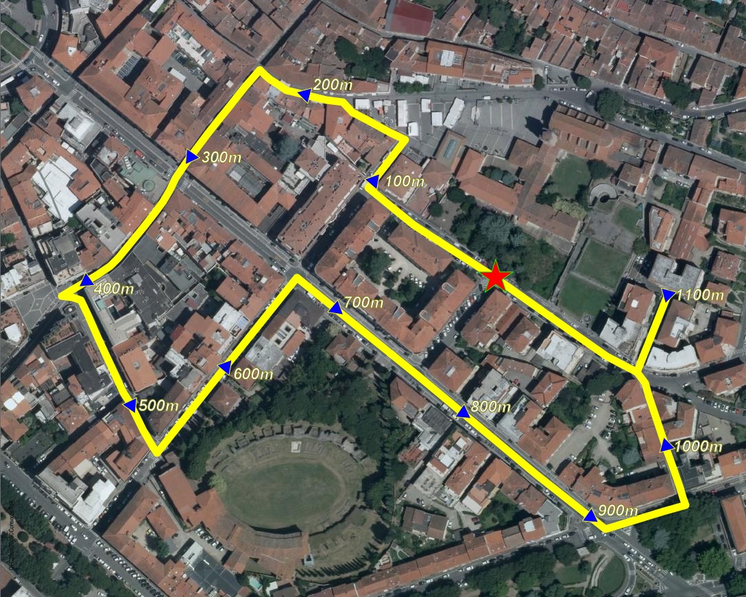
The map below graphically shows the previous multi-destinations queries.
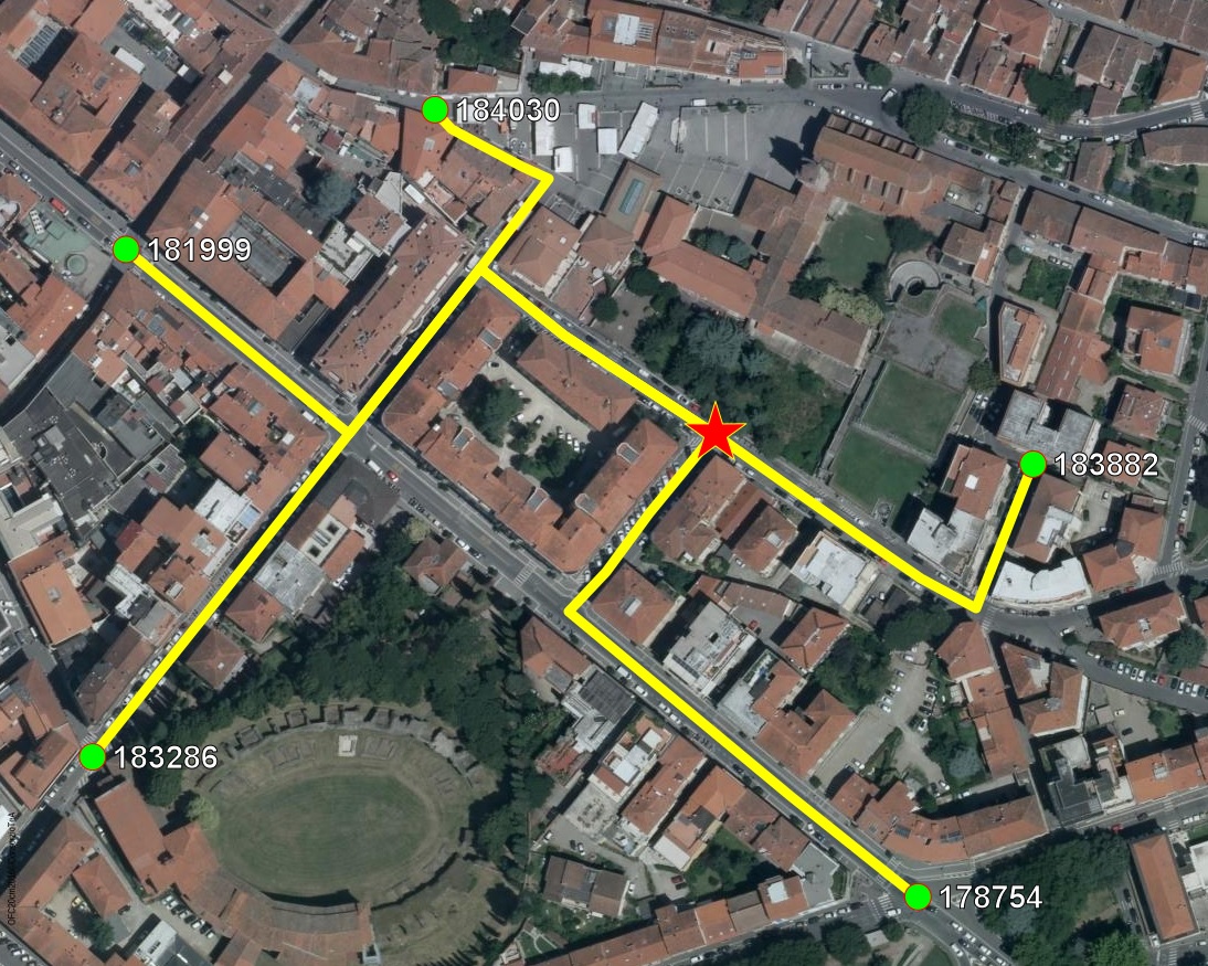
- Red star: the Origin Node.
- Green dots: the Destination Nodes.
- Yellow lines: all individual travel solutions.
Dangerous pitfalls related to multiple destination listsSQL syntax directly allows to specify lists of multiple values, so may be you are now wondering about writing the multiple destinations query tested in the previous examples this way:SELECT Algorithm, Request, Options, Delimiter, RouteId, RouteRow, Role, LinkRowid, NodeFrom, NodeTo, Cost, Geometry, Name FROM byfoot WHERE NodeFrom = 178731 AND NodeTo IN (183286, 290458, 181999, 184030, 124622, 183882, 178754);There is a very good reason discouraging from doing such a thing, let's see why. SQLite will process a request written this way by repeatedly calling VirtualRouting passing each time a single Destination; and consequently VirtualRouting will never receive the critical information that a single monolithic request was intended to be executed in a single shot. So the request context will be easily misinterpreted, and any expected speed benefit will be completely frustrated. BewareNever ever attempt to define a list of multiple destinations using the standard SQL syntax WHERE NodeTo IN (......), because this will certainly cause many unexpected troubles.Badly formatted resultsets will be then returned, may be containing wrong results. You are warned. |
How to correctly format multiple destinations listsVirtualRouting always expects to receive a multi-destinations list as a TEXT string containing tightly packed values separated by a conventional delimiter (usually represented by a comma).Examples of well formatted multi-destinations lists: '1,2,3,4,5,10,100,1000,100000' -- integer Node IDs 'A100B,A100F,B250Z,C010M,Z999A' -- alphanumeric Node CodesExamples of badly formatted multi-destinations lists: ' 1, 2, 3, 4 , 5 , 10, 100, 1000, 100000 ' -- integer Node IDs ' A100B, A100F , B250Z , C010M, Z999A ' -- alphanumeric Node CodesNote: all whitespaces immediately preceding or following the delimiter will be considered to be integral part of the value itself. This will have no adverse consequences in the case of integer values, but can easily have catastrophic effects on alphanumeric values. Defining a custom delimiterSometimes it could be useful setting up a delimiter different from comma.UPDATE byfoot SET Delimiter = '*'; SELECT Delimiter FROM byfoot; ------------------ * [dec=42, hex=2a]You simply have to execute an UPDATE statement by specifying the new delimiter value. |
6 - Solving TSP (traveling salesman) problems
TSP (Traveling Salesmn Problem) is a well known Operations Reasearch problem.
The Traveling Salesman ProblemGiven a list of cities and the distances between each pair of cities, what is the shortest possible route that visits each city and returns to the origin city ? |
Note: the terms salesman and city are universally used for historical reasons, but you should avoid to literally intend both them.
The term salesman in this specific contest intends any possible kind of moving agent (pedestrian, vehicle, passenger or whatever else), exactly as city simply stands for any generic destination on a given Network.
We can concettualy split TPS in two halves:
- computing all distances beteen pairs of cities.
this is a typical ShortestPath problem, and we can duly use the Dijkstra's algorithm for this. - then we have to check all possible permutations / combinations so to identify the optimal TSP solution.
Simply computing the complete TSP solution for about ten cities will require a very long time even using a supercomputer.
And attempting to compute a TSP solution for about hundred cities will require a practically infinite time.
However solving TSP is highly desiderable in many application fields: logistics (just think about courier companies as DHL, FedEX, UPS or TNT), field maintenance, waste collection, schoolbus / shared taxi services etc.
Many algorithms have been invented during last decades intended to produce practical although approximate / imperfect TSP solutions in a reasonably short time. Many of them strongly depend on heuristic and / or randomness.
VirtualRouting supports two different TSP algorithms:
- TSP NN (aka Nearest Neighbour)
This first algorithm is straightforwad simple and very fast; it can effectively solve huge TSP solutions (thousand cities or even more) in a very short time.
Short description:- starting from the base city the salesman goes to the city presenting the lesser connection cost.
- the already visited city is cancelled from the list, and then the salesman goes to the next city presenting the lesser connection cost.
- the cycle continues until all cities in the list have been visited.
- finally, the salesman returns to his/her initial base city
In the most unlucky case TSP NN could possibly return the worst solution, but the specific implementation adopted by VirtualRouting checks against this possibility:- each TSP NN is always computed twice by randomly choosing a different base city and then normalizing the solution; the best of the two solutions is then returned.
- this simple but effective precaution robustly ensures that the worst solution will never be returned, and just implies a moderately increased execution time.
- TSP GA (aka Genetic Algorithm).
This alternative algorithm is much more complex and sophisticated, and is directly inspired by biological concepts such as sexual reproduction, genetic mutations and natual selection.
Short description:- a first initial set of solutions (the population) is created by using TSP NN after randomly choosing the base city and then normalizing each solution.
- then during each step of the execution loop (generation) pairs of solutions sexually reproduces giving birth to children solutions; chromosome crossovers and random mutations intrinsically affect the reproductive process.
- for each generation the natural selection eliminates all poorly fit individuals from the population and consequently only the best fit individuals can propagate their genome to next generation.
- after a certain number of generations (let's say about some hundredth iterations) the optimal solution (or at least a fairly good sub-optimal solution) should finally emerge, and so the loop can exit.
- Note: TSP GA is usually expected to identify better solutions than TSP NN can do, but it will surely require much more time to complete.
Let's now examine a practical example of TSP solving using VirtualRouting.
UPDATE byfoot SET Request = 'TSP';

SELECT Algorithm, Request, Options, Delimiter, RouteId, RouteRow, Role, LinkRowid, NodeFrom, NodeTo, Cost, Geometry, Name
FROM byfoot
WHERE NodeFrom = 178731 AND NodeTo = '183286,181999,184030,183882,178754';
A VirtualRouting TSP query has the same identical form of a multi-destination query; the base city is always expected to correspond to NodeFrom and all other cities to be visited are expected to be enumerated into a multi-destination list assigned to NodeTo. Note: you must explicitly set the current Request as TSP, TSP NN or TSP GA (TSP and TSP NN are synonims).
| Algorithm | Request | Options | Delimiter | RouteId | RouteRow | Role | LinkRowid | NodeFrom | NodeTo | Cost | Geometry | Name |
|---|---|---|---|---|---|---|---|---|---|---|---|---|
| Dijkstra | TSP NN | Full | , [dec=44, hex=2c] | 0 | 0 | TSP Solution | NULL | 178731 | 178731 | 1254.433933 | BLOB sz=2000 GEOMETRY | NULL |
| NULL | NULL | NULL | NULL | 1 | 0 | Route | NULL | 178731 | 184030 | 176.364755 | BLOB sz=304 GEOMETRY | NULL |
| NULL | NULL | NULL | NULL | 2 | 1 | Link | 224014 | 178731 | 182885 | 94.812424 | NULL | VIA PIETRO ARETINO |
| NULL | NULL | NULL | NULL | 2 | 2 | Link | 224862 | 182885 | 182043 | 37.095287 | NULL | VIA MARGARITONE |
| NULL | NULL | NULL | NULL | 2 | 3 | Link | 226070 | 182043 | 184030 | 44.457044 | NULL | PIAZZA SANT'AGOSTINO |
| NULL | NULL | NULL | NULL | 2 | 0 | Route | NULL | 184030 | 181999 | 139.114938 | BLOB sz=496 GEOMETRY | NULL |
| NULL | NULL | NULL | NULL | 3 | 1 | Link | 226071 | 184030 | 182629 | 55.689009 | NULL | VIA GIUSEPPE GARIBALDI |
| NULL | NULL | NULL | NULL | 3 | 2 | Link | 225512 | 182629 | 182933 | 34.184194 | NULL | CORSO ITALIA |
| NULL | NULL | NULL | NULL | 3 | 3 | Link | 225511 | 182933 | 181999 | 49.241735 | NULL | CORSO ITALIA |
| NULL | NULL | NULL | NULL | 3 | 0 | Route | NULL | 181999 | 183286 | 217.672885 | BLOB sz=688 GEOMETRY | NULL |
| NULL | NULL | NULL | NULL | 4 | 1 | Link | 222635 | 181999 | 181998 | 101.629750 | NULL | CORSO ITALIA |
| NULL | NULL | NULL | NULL | 4 | 2 | Link | 224780 | 181998 | 183560 | 73.733572 | NULL | VIA DELL'ANFITEATRO |
| NULL | NULL | NULL | NULL | 4 | 3 | Link | 225827 | 183560 | 183286 | 42.309564 | NULL | VIA DELL'ANFITEATRO |
| NULL | NULL | NULL | NULL | 4 | 0 | Route | NULL | 183286 | 178754 | 378.313684 | BLOB sz=272 GEOMETRY | NULL |
| NULL | NULL | NULL | NULL | 5 | 1 | Link | 224414 | 183286 | 178880 | 136.372057 | NULL | VIA MARGARITONE |
| NULL | NULL | NULL | NULL | 5 | 2 | Link | 219171 | 178880 | 178732 | 93.285538 | NULL | VIA FRANCESCO CRISPI |
| NULL | NULL | NULL | NULL | 5 | 3 | Link | 219058 | 178732 | 178754 | 148.656089 | NULL | VIA FRANCESCO CRISPI |
| NULL | NULL | NULL | NULL | 5 | 0 | Route | NULL | 178754 | 183882 | 188.216831 | BLOB sz=400 GEOMETRY | NULL |
| NULL | NULL | NULL | NULL | 6 | 1 | Link | 224538 | 178754 | 181972 | 50.900663 | NULL | VIA ANTONIO GUADAGNOLI |
| NULL | NULL | NULL | NULL | 6 | 2 | Link | 224537 | 181972 | 182000 | 86.301051 | NULL | VIA DEL NINFEO |
| NULL | NULL | NULL | NULL | 6 | 3 | Link | 225527 | 182000 | 183882 | 51.015117 | NULL | VIA LICIO NENCETTI |
| NULL | NULL | NULL | NULL | 6 | 0 | Route | NULL | 183882 | 178731 | 154.750839 | BLOB sz=240 GEOMETRY | NULL |
| NULL | NULL | NULL | NULL | 7 | 1 | Link | 225527 | 183882 | 182000 | 51.015117 | NULL | VIA LICIO NENCETTI |
| NULL | NULL | NULL | NULL | 7 | 2 | Link | 222636 | 182000 | 178731 | 103.735722 | NULL | VIA PIETRO ARETINO |
Let's now quickly examine the resultset returned by any TSP query:
- the general layout is more or less the same as you've already seen in the case of ShortestPath queries, but in this specifc case it represents the TSP solution as a whole.
- the first row of the resultset is someway exceptional, and is the unique row of the resultset presenting NOT NULL values in the Algorithm, Request, Options and Delimiter columns.
- columns RouteId and RouteRow have the same interpretation as in multi-destination ShortestPath queries, but in this specific case each route corresponds to a connection between two cities.
All routes are order accordingly to the running sequence of the TSP solution.
UPDATE byfoot SET Request = 'TSP GA';

SELECT Algorithm, Request, Options, Delimiter, RouteId, RouteRow, Role, LinkRowid, NodeFrom, NodeTo, Cost, Geometry, Name
FROM byfoot
WHERE NodeFrom = 178731 AND NodeTo = '183286,181999,184030,183882,178754';
If you whish to get a TSP GA solution you simple have to set Request as TSP GA; and you can set again Request as TSP or TSP NN to revert back to the simpler / faster algorithm.
The map below graphically shows the previous TSP query.
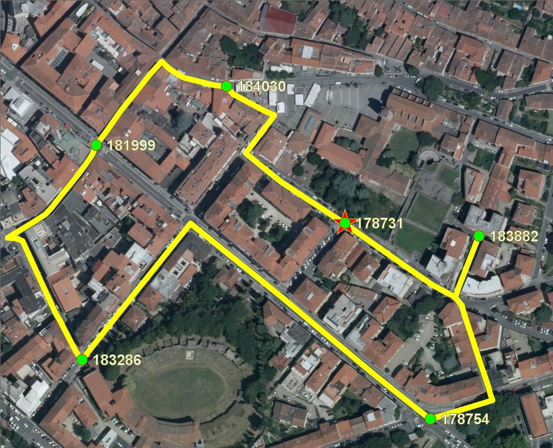
- Red star: the base-city (i.e. from where the salesman</b<) begins his/her trip.
- Green dots: the cities to be visited.
- Yellow line: the TSP solution (that is always a circular path).